Consumer Demand
Foundations of microeconomics start with how consumers behave. We might want to predict what a consumer is likely to do in a given situation. We might want to make sense of observed behavior. The theory will appear simplistic. But from this simple theory, we will be able to predict pretty well behavior in certain situations. Refinements exist, in particular to allow consumers to be more humans, have biases, cognitive limitations, emotions.

Preferences
Preferences are defined over baskets of goods and services
Basket: vector of quantities \(x = (x_1, x_2,\cdots,x_n)\).
For any baskets \(A\) and \(B\), preferences dictate which one is preferred.
Preferences are just like wish lists. They ignore prices and resources.
Preference relations are denoted \(\succ,\succeq,\sim\).
Important assumptions about preferences
Assumptions (or axioms as they are called) on preferences are necessary to yield a theory of how consumers behavior. These axioms yield predictions. Among the most important, we have that they should be:
Exhaustive
For any two baskets A and B, either the consumer:
prefers always A to B (\(A\succ B\))
prefers always B to A (\(B\succ A\))
is indifferent between A and B (\(A \sim B\))
Is it restrictive?
Yes, e.g.: ice cream vs. soup (one prefers ice cream in summer but soup in winter).
But we can accommodate include circumstances in the preferences (the season)
Baskets are now (ice cream, summer), (ice cream, winter, (soup, winter), (soup, summer). The preference relation may now be stable and exhaustive.
Transitivity
Given three baskets A, B, C such that \(A\succ B\), \(B \succ C\), then if transitivity holds he also prefers A to C (\(A \succ C\)).
This assumption appears logical. But it sometimes fails. In particular when uncertainty is present. Yet, we will keep it as it is very important for what follows.
Non-satiation
In its simplest form, this assumption implies that
If A has the same quantity of each good as basket B, but strictly more of one good, then \(A \succ B\).
Weaker version (\(A \succeq B\),indifference or preference) is reasonable.
Putting labels on goods so non-satiation makes sense: goods are typically labeled as desirable (air quality instead of pollution).
It is not practical to use wish lists to model behavior. For example, how do we predict how consumers react to price changes using a wish list? We will want to get closer to marginal analysis to make this more practical.
Finally, it is important to note that preferences are very different across consumers. Falk et al. (2018) have analyzed this heterogeneity in 76 countries.
Indifference Curves
One of the first tools we can construct is indifference curves.
For any two goods \(X,Y\):
Starting from a basket \((X_0,Y_0)\), find combinations of \((X,Y)\) such that the consumer is indifferent between \((X,Y)\) and \((X_0,Y_0)\)
In the plane (\(X,Y\)), higher indifference curves indicate a preference.
Proposition: If transitivity holds, indifference curves cannot cross.
Exercise A: Show that this last proposition is correct.
Marginal Rate of Substitution (MRS)
These indifference curves contain more information than we think …
For a basket \((X_0, Y_0)\), MRS of \(X\) in terms of \(Y\): Quantity of good \(Y\) the consumer is willing to sacrifice to increase \(X\) by one unit.
Marginal value the consumer puts on \(X\) in terms of quantity of good \(Y\).
Corresponds to the slope at \((X_0,Y_0)\).
Convexity of indifference curves
If the quantity of \(X\) increases, how does the MRS for \(X\) changes?
It decreases generally. This implies convex indifference curves. Even if there is non-satiation, we generally accept that the intensity of preference decreases as the quantity consumed increases.
Utility
Indifference curves allow us to move away from wish lists to a function. On an indifference curve, each basket gives the same level of satisfaction to the consumer (he is indifferent). Let’s fix that level to some arbitrary number, called utility. Jumping from one indifference curve to another change the level of satisfaction. Hence, indifference curves are like level curves on a topological map, they do not cross. The main insight is that we can construct a function \(U(X,Y)\) which represent these preferences. The value of this function is ordinal, it allows to rank the different indifference curves. It is only this order that counts.
Utility function: assigns a value to each basket. \(U\) represents these preferences if \(A \succ B \Rightarrow U(A) > U(B)\) and \(U(A) > U(B) \Rightarrow A \succ B\) for any two baskets.
This has a number of implications. The main one is that there are many utility functions that represent the same preferences…
If \(f\) is a strictly increasing transformation (function) and \(U\) represents some preferences, then \(V(X) = f(U(X))\) represents the same preferences.
\[U(X) > U(Y) \iff f(U(X)) > f(U(Y))\]
In other words, the value attached to utility does not have a real interpretation, it is the ranking of baskets through the level of these utility levels which matters.
Example: \(U(X,Y) = \log X + \log Y\) and \(V(X,Y) = XY\) represent the same preferences.
Exercise B: Show that \(U\) and \(V\) in this example have the same preferences by finding the transformation \(V=f(U)\).
How to find the MRS from utility?
Two goods, \(X\), \(Y\). Preferences are represented by \(U(X,Y)\)
e.g. \(U(X,Y) = \log X + \log Y\)
MRS of \(X\):
How much \(Y\) should one sacrifice to gain \(X\)
Formally: if we increase \(X\) by \(\Delta X\): what is the change \(\Delta Y\) which maintains indifference?
We can use total differentiation:
Set \(dU = 0\). Then
Budget Constraint
Until now, the consumer has available all baskets and he has preferences over those. In practice, he is limited by the resources he has, each time he has to purchase goods, at some price. Hence, those actions have an opportunity cost.
One cannot spend more than income (or wealth) \(I\)
- Two goods \(X\), \(Y\): Constraint: \(p_X X + p_Y Y \leq I\). This constraint determines what is available given \(I\) and prices.
- Setting to equality, we can solve for \(Y\) in terms of \(X\): \(Y = \frac{I - p_X X}{p_Y}\)The relative price between \(X\) et \(Y\) holding the budget constant is:\[\frac{dY}{dX} = -\frac{p_X}{p_Y}\]
Buying a unit of \(X\) implies a sacrifice of \(\frac{p_X}{p_Y}\) units of \(Y\). It is the opportunity cost of \(X\) in terms of \(Y\).
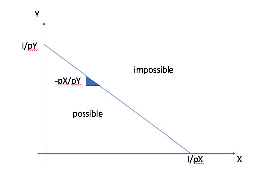
In the space \((X,Y)\), the budget line defines all possible allocation. Those above are not feasible. Those on the line or below are feasible.
Normalization
The budget constraint remains the same if we multiply prices and income by the same constant \(\lambda\).
One can buy the same goods. Hence, currencies do not impact the budget constraint. Only purchasing power and relative prices do.
Therefore we will sometimes set \(p_Y = 1\). Then \(Y = I - p_X X\). \(p_X\) is in terms of the quantity of \(Y\) (numéraire) and idem pour \(I\).
Only relative prices matter.
Exercice C: Show that the budget constraint does not change if we multiply prices and income by \(\lambda>0\).
Consumer choice
The constraint is a given and therefore fixed. The consumer can pick on which indifference curve he wants to be and where on that curve. It seems natural to predict that he will want to pick the feasible basket which maximizes his utility.
He can’t go on an indifference curve above the budget line.
Those allocations below the budget line cannot be optimal if we have non-satiation. He has money to spare and could spend it on goods which provide (marginal) utility.
The indifference curve that touches on the constraint (tangent) gives the highest feasible level of utility.
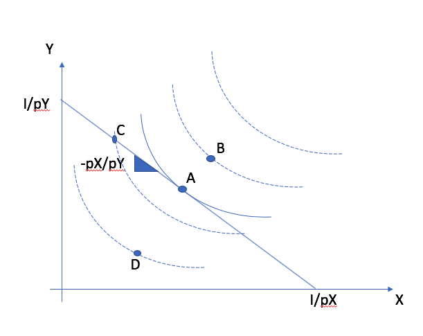
The points A, C et D are possible given the constraint. Therefore, point B can be eliminated even if the MRS (slope at B) is close to the price ratio. Point D can also be eliminated because the consumer does not spend all his budget. He can jump on a higher indifference curve by increasing consumption of each good. Bundles A and C spend exhaust the budget. But C is not optimal. In absolute terms, the MRS is larger than the opportunity cost (price ratio) of consuming another unit of X. Therefore, she can increase X and reduce Y yielding higher utility. Point A is optimal: MRS is equal to the price ratio.
Direct approach
The problem is
Maximize \(U(X,Y)\) given the constraint \(p_X X+ p_YY = I\)
Step 1: Substitute the constraint
If buys \(X\) can consume \(Y(X) = \frac{I - p_X X}{p_Y}\)
Utility now function of \(X\) only: \(V(X) = U(X,Y(X))\)
Step 2: Maximize unconstrained
Look at first order condition (FOC)
The FOC is:
\[\frac{dV}{dX} = 0 \iff \frac{dU}{dX} + \frac{dY}{dX}\frac{dU}{dY} = 0\]\[\iff \frac{dU}{dX}\Bigg/\frac{dU}{dY} = \frac{p_X}{p_Y}\]
MRS equal to relative price comes out naturally as FOC.
Exercise D: Find demands for \(u(x,y) = XY\) under the constraint \(p_X X + p_Y Y \le I\).
As an alternative, we can set up the Lagrangian:
The constrained problem is therefore \(\max_{X,Y,\lambda} L(X,Y,\lambda)\). The FOCs are
Taking the ratio of the first two FOC (after sending price terms to rhs), we get:
Hence, MRS equal to price ratio and budget constraint met are the two conditions for an optimum.
Exercice E: Find demands for \(u(X,Y) = XY\) using the Lagrangian.
Demand functions \(X^*(p_X,p_Y,I)\) and \(Y^*(p_X,p_Y,I)\) are called Marshallian demands (Alfred Marshall).
Indirect utility
Indirect utility \(V(p_X,p_Y,I)\) is the maximum level of utility the consumer can reach with prices \((p_X,p_Y)\) and income \(I\),
Now a number of key points can be made about this function. The first is that the Lagrange multiplier has an interpretation:
By definition,
Hence, the derivative with respect to \(I\) is
where I subindices denote partial derivatives and we omit arguments for brevity. We can collect terms to get
Now from the FOC to the Lagrangian, the first and second terms are zero at the optimum (\(U_X - p_X \lambda=0\) and \(U_Y - p_Y \lambda=0\)), yielding
The marginal utility of income in a static consumer choice problem is the Lagrange multiplier. An important mathematical note: the result above where the two terms involving the FOC cancel out is due to a well-known theorem in constrained optimization: the envelope theorem. We will refer to it a few times. In words, it states that when evaluating the derivative of the objective function at the optimum with respect to one of the exogenous variables (say a price or income), one does not need to look at re-optimization (the fact that the optimal decisions change). Only the envelope matters: how the function changes directly as a function of the exogenous variables. The logic is simple: Given a derivative look at a very small change, the induced change to the optimal solution has an effect on the objective function that is small and zero by the FOC. This only works for small changes.
Roy Identity
Given the indirect utility function \(V(p_X,p_Y,I)\) we can retrieve demand functions using:
Exercice G: Show that this is true using the envelope theorem.
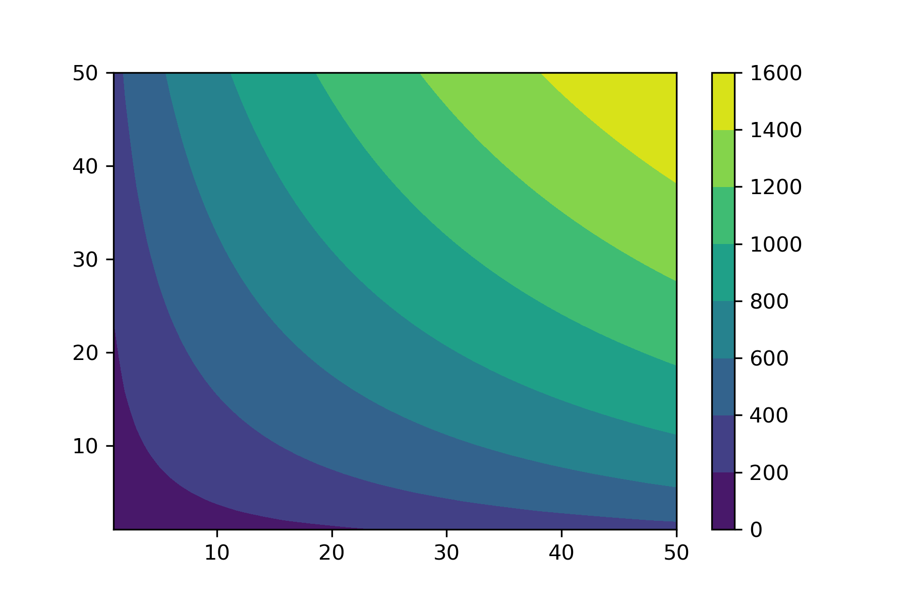
Consumer Demand Example
See this example in Python for a special utility function that is often used in practice: the CES (Constant Elasticity of Substitution)
![]()