Labor Supply
The consumer problem has so far been focused on picking consumption goods. Income is exogenous. In reality, our income is not exogenous. We can decide to work more or less to change our income. When we do, we reduce or increase the time we denote to leisure. We can think of leisure as a consumption good. Increasing income, by working more, has an opportunity cost in terms of leisure foregone. In this class, we focus on this margin.
Many questions can be addressed in this setting: how does subsidized childcare impact labor supply of mothers? How can we make older workers stay longer in the labor force? What are the impacts of replacing our social programs with a guaranteed minimum income.
Model
To model this choice, we introduce a new good, leisure time \(L\). Time available each day (effective after subtracting time to sleep and personal care) is given by \(T\). Therefore, time devoted to work is given by \(H=T-L\). Here, we assume that there are only two uses of our time: leisure and work. It is possible to introduce more, for example home production of goods. The Nobel laureate Gary Becker has been one of the pioneers in the economic analysis time allocation.
The consumer has preferences for \((C,L)\), where \(C\) is consumption goods (we normalize the price to 1) and \(L\) is leisure time (per day, week or years), represented by \(u(C,L)\), generally concave in its two arguments. The MRS between consumption and leisure is given by:
and represents, in absolute value, the marginal value granted to an hour of leisure. Leisure has a positive value.
When she works, the consumer has an hourly wage \(w\) and other income \(y\). If she works \(H=T\) hours, she has a full income of \(I = w T + y\). She implicitely spends on two goods she consumes, \(C\) and \(L\). Leisure has the opportunity cost per hour worked given by \(w\). The budget constraint is given by:
Note that both spending and full income is a function of \(w\). We can rewrite the constraint using \(H=T-L\):
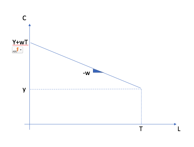
The budget constraint, in the space \((C,L)\) is kinked because of the presence of \(y\) and has a slope \(-w\).
The labor supply problem can be written as a Lagrangian:
The FOCs are
The first condition states that the absolute value of the MRS (marginal value of an hour of leisure) is equal to its opportunity cost. The second condition is the budget constraint. The solution to this system gives marshallian demands for consumption and for leisure, \(L^*(w,y)\). Labor supply is given by \(H^*(w,y) = T - L^*(w,y)\).
Exercise A: Find the demand for leisure and labor supply for \(u(C,L) = C^{\alpha}L^{1-\alpha}\).
The Lagrange multiplier has an interpretation as marginal utility of income. We also need to realize that the presence of \(y\) may result in a corner solution where \(L^* = T\) and the MRS is larger than the wage.
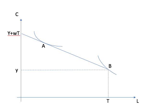
The situation A shows a labor supply choice with higher hours of work than situation B which shows a situation where the worker does not work (corner solution. In this case, the MRS is larger than the wage \(L=T\).
Substitution and Income Effects
The presence of \(w\) in full income, which makes the analysis of wage changes more challenging. An increase in the wage now increases the opportunity cost (leading to a substitution effect) but also increases full income (making leisure more desirable if leisure is a normal good).
To understand these effects, we first note that the choice problem can be rewritten to involve only one decision, leisure time, by substituting the budget constraint,
The FOC is:
where \(u_C\) is the marginal utility of consumption and \(u_L\), the marginal utility of leisure. Total differentiating and setting \(dy=0\), we get
where \(\Delta\) is negative. Hence, the effect of a change in the wage is the sum of a negative term (first term) and a positive income effect term (if leisure is normal). The effect of a wage change on leisure is undetermined and will depend on the relative strength of these two effects.
We can re-write to obtain a Slutsky equation for labor supply by first rewriting in terms of hours worked:
The substitution effect is now positive and the income effect negative. In terms of elasticity, we have
We can estimate the wage and income elasticity in different ways. For example, Imbens et al. (2001) estimate the income elasticity from looking at lottery winners. This allows to estimate \(\eta_{Y}\). They find an income elasticity between -0.05 and -0.1.
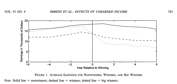
Imbens et al. (2001)
For wage elasticity, the literature is vast. Generally, the elasticity is smaller for men, larger for women, in particular for the choice of entering the labor market or not.
Exercise B: Find the wage elasticity and compensated wage elasticity for \(u(C,H) = C - \frac{H^{1+\frac{1}{\epsilon}}}{1+\frac{1}{\epsilon}}\).
It is possible that a wage increase leads to a reduction of hours worked. This happens when the income effect dominates the substitution effect. This can be observed in certain occupations. Physician labor supply is the prime example. After large increases in salaries, the fraction of physicians working part-time has increased substantially.
A particular case which involves an income effect that is exactly equal to the substitution effect (in absolute terms) is income targeting. This study on taxi drivers in New York is a good example.
Taxation
Taxation can take many forms. In its simplest form, it is a tax rate \(\tau\) on work income. If we look at the budget constraint, we have
Therefore, increasing the tax rate is similar to reducing the wage. We denote the after-tax wage as the net wage. Since we know that the effect of a change in wages has an undetermined effect, it is therefore not possible in general to put a sign on the effect of a change in work income taxation.
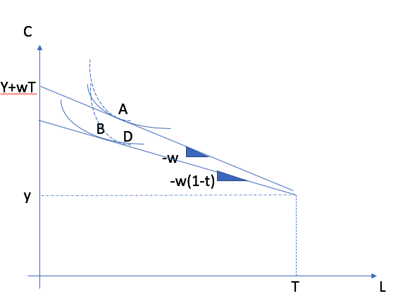
Relative to a baseline A, the effect of the tax depends on the shape of indifference curves. It is possible that the worker works less (situation D, substitution effect dominates) or more (situation B, income effect dominates).
In addition, the implementation of the tax is important to assess the change. The more permanent is a tax, the more workers will feel the income effect while if a tax is transitory, the substitution effect is likely more important. Furthermore, if there is compensation, for example for low wage earnings, this needs to be taken into account and the compensated wage elasticity should be used.
The bottom line is that the effect of taxes on labor supply is far from trivial and depends on a multitude of dimensions.
Exercise C: In the case where preferences are given by \(u(C,H) = C - \frac{H^{1+\frac{1}{\epsilon}}}{1+\frac{1}{\epsilon}}\), find the effect of a tax \(\tau\) on labor supply and the welfare loss associated with taxation.
In reality, the tax system cannot be summarized by a single tax rate \(\tau\). First, income taxes are progressive and the marginal tax rate changes across tax brackets. In addition, income tax credits impact the effective marginal tax rate since they are often function of work income. Generalizing, taxes paid are a function \(\tau(wH,y)\) which depend on sources of income tax and the level.
One such measure that is useful is the effective marginal tax rate (EMTR). It can be computed as
The EMTR is useful to measure the effective marginal tax rate one will pay when working an additional hour. In the Python example below, you will compute such measures for a worker in Quebec.
An interesting method for assessing the effect of taxation is to look for bunching at places where the effective marginal tax rate changes abruptly. The American study of Saez (2010) is a good example of a bunching study. They find bunching in the first income tax bracket but not for other tax brackets.
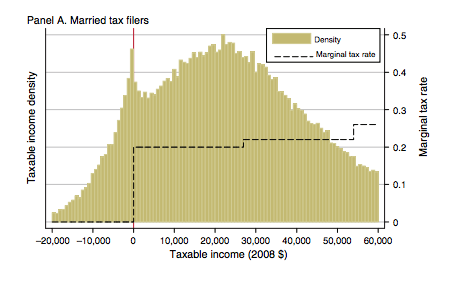
Saez (2010)
Transfers
Governments provide transfers to households with low income. These transfers impact choices in the same way that \(y\) does. Therefore, they have primarily an income effect in household behavior and increase the likelihood of a corner solution (zero hours worked).
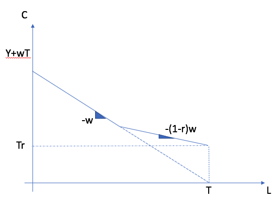
In addition, they can have substitution effects since transfers are often taken away (clawed back) when work income increases. They can therefore increase EMTRs when someone attempts to exit low-income status. If badly designed, these transfers can act as a poverty trap.
Social assistance in Quebec is reduced dollar for dollar. This is a 100% implicit tax rate. Another benefit that counters that effect is the work income tax credit (prime au travail in Quebec). It first increases as the first dollars are earned and then reduced. Overall, the design of a good transfer system that provides good coverage for low-income households and incentives to return to work is not a simple task.
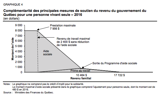
Source: Final report, Comité sur le revenu minimum garanti, Volumne 2.
Graphically, we end up with a budget constraint that looks like this when transfers are clawed back.
If it is hard with the preferences in the figure to incentivize return to work with the transfer provided. The incentive to return is not there.
Question for discussion: For or against a guaranteed minimum income, in particular to help people get out of poverty? What do you need as economists to answer this question?
Background reading for discussion:
Report from the Expert committee on basic income.
Survey results on support for UBI

