Imperfect Competition
Situations where firms operate in perfect competition, as price takers, do arise but there are plenty of other situations where firms have market power. Many markets have a few firms. Having few firms is not a perfect signal that firms have market power, but it creates the conditions for strategic behavior. We will try and analyze these situations. Analyzing imperfect competition involves looking more closely at the strategy of firms.
Perfect Competition
General equilibrium with production, the topic of the previous lecture, assumes that firms are price takers. This leads to a market equilibrium with the first welfare theorem applying. It is a Pareto optimum. This assumption of price-taking behavior works well when a very large number of firms are present. Firms cannot impact the market price by their actions. We will see that it is the possibility of affecting the market price which confers to the firm market power.
Consider the example of an economy for a good \(X\) and a numéraire good \(M\) (with a normalized price to one). Utility is quasi-linear \(U(X,M) = V(X) + M\), with \(V(X)\) concave, \(V'(0) = + \infty\). Endowments are \(I_0\) of \(M\), the good \(X\) is produced by one firm at price \(p\). The firm is producing \(X\) with a cost function \(C(X)\). Assume \(C'(0) = 0\).
Exercise A Find the equilibrium price if the firm is a price taker and \(V(X) = \sqrt{X}\), \(C(X) = X^2\).
Given production at some price, producer surplus is given by:
When there are no fixed costs, this is equivalent to profits. Note that if a firm faces a constant marginal cost, producer surplus in a perfectly competitive market equilibrium is zero. With increasing marginal cost (decreasing returns to scale), profits are positive but the marginal unit produced in equilibrium brings in zero profits.
Strategic Price Manipulation
Firms who by their production choices impact the equilibrium price have market power. They can generate more profits relative to the perfect competition situation. The firm can reduce production, below the quantity which is Pareto optimal in perfect competition. This leads to an equilibrium price above marginal cost (the price is set when marginal revenue equals marginal cost). This increases profits of the firm.
To understand this strategic behavior, observe that the firm picks \(X\) to maximize
\[\Pi = p(X)X - C(X)\]
The FOC is
\[\frac{d\Pi}{dX} = 0 \iff p'(X)X + p(X) = C'(X)\]
which leads to a choice \(X_{PM}\) such that
The left-hand side is marginal revenue while the right-hand side is marginal cost. The first term on the left is the marginal effect of an increase in the quantity. The marginal unit produced brings in \(p(X_{PM})\). This effect is the only one showing up when the firm is a price taker. The quantity chosen is such that the price (marginal revenue) is equal to marginal cost.
But a second term is present on the left-hand side. There is an infra-marginal effect on marginal revenue when actions impact the price. When the firm increases quantity, the market price goes down (no Giffen good). Therefore, the revenue it receives from producing what it already produces \(X_{PM}\) goes down.This effect is negative since \(p'(\cdot)\) is negative. Overall, marginal revenue is the sum of a positive and a negative term, hence lower than when the firm is a price taker. At the price-taker quantity produced, the marginal revenue is lower than marginal cost. The firm will reduce the quantity produced to restore equality and maximize profits.
Exercise B Find the equilibrium price if the firm strategically manipulates the price and \(V(X) = \sqrt{X}\), \(C(X) = X^2\). Show in a graph that situation relative to the price taker situation.
Exercise C : In exercise B, find the expression for the equilibrium price as a function of the price elasticity of demand. Analyze that situation.
The Inverse Problem It is also possible to write the strategic price manipulation problem in terms of a choice over price rather than quantity. This leads to the same result but viewed from the explicit choice of prices. For example, let \(X(p)\) be demand (instead of inverse demand). With constant marginal cost, we get
The FOC is
which can be solve for the optimal price given a demand function \(X(p)\).
A few market configurations are associated with market power and therefore strategic behavior.
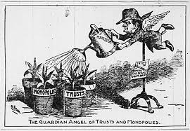
Monopoly
A monopoly exists when one firm is in a market. If demand is not perfectly elastic, the monopoly can manipulate the price strategically by changing its production level and increase profits.
At the optimal level of production \(X_{PM}\) we have
\[p(X_{PM}) + p'(X_{PM})X_{PM} = C'(X_{PM})\]
and therefore if \(p'(X_{PM})<0\), then \(p(X_{PM}) > C'(X_{PM})\).
The monopoly picks a production level which leads to a higher price than marginal cost. If production does not have an impact on the price, the firm is a price taker and produces \(X_{PT}\) at \(p(X_{PT}) = C'(X_{PT})\). Therefore, \(X_{PM} < X_{PT}\).
To perform weflare analysis, we first have to ask why the monopoly exists. He can either be articifial because barriers to entry exist or natural because large economies of scale exist. The case we consider here is one where barriers to entry create this situation. For example, this could arise because of regulation (the firm is allowed to be alone on the market) or technological constraints. A firm could own the infrastructure to bring the internet to a particular region and others need to pay to use that infrastructure. If the price is set high enough, this creates barriers to entry. Generally speaking, this type of monopoly situation will lead to a welfare loss.
Other situations are more complicated. Take electricity. Because of large fixed costs, there are important returns to scale in producing electricity. These efficiency gains from granting a monopoly need to be compared to the loss from market power and other disincentives which may be present with monopolies not facing competition (e.g. innovation or cost control).
In the case of an artificial monopoly, it potentially makes abnormal profits, called rents. These profits are given by
\[\Pi_{PM} = (p(X_{PM}) - p(X_{PT})) X_{PM}\]
Rents reduce consumer surplus for units produced by the monopoly. But these rents are not the source of the welfare loss. The welfare loss occurs on units not produced or consumed, because of the monopoly situation. These units have positive economic value \(V'(X)-C'(X)>0\).
Exercise D: Show monopoly rents and the welfare loss in the graph made for Exercise B.
Duopoly
We use the term duopoly to denote a market with two firms and oligopoly with a small number of firms (including 2). In this section, we focus on the case with two firms.
To build a model of how these firms interact, we must choose whether they compete on quantities or price. In a situation where capacity is an issue, where it takes time to produce, competition typically occurs on quantity. Think of industrial machinery, planes, trains. In situations where capacity is not an issue, competition will occur on price. One firm could supply the entire market and adjustment is fast. Think of retail as a good example, Competition on quantity is often denoted Cournot competition. Competition on prices is denoted Bertrand competition. Both have very different implications.
Cournot
Cournot competition is done on quantities produced. Commercial airliner production is the classical example with the battle between Boeing and Airbus. Producing a plane is costly and production cannot be adjusted rapidly. The decision to produce is a strategic decision.
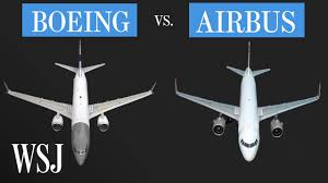
Source: The Wall Street Journal.
We can consider, without loss of generality, the case of two identical (symmetric) firms producing \(X_A\) and \(X_B\).
Consumers have preferences represented by \(U(X,M) =V(X) + M\). More specifically,
\[V(X) = D_0 X - \frac{\alpha}{2} X^2\]
Costs of these two firms are represented by \(C_A(X) = C_B(X)= c X\). Using quasi-linear preferences with a quadratic valuation function is useful as the inverse demand is given by \(P(X) = V'(X) = D_0 - \alpha X\).
What is the correct benchmark in this situation? A natural choice is the Pareto optimal outcome for consumers.
The optimal quantity would be \(X\) such that the marginal cost is equal to the marginal willingness to pay from consumers:
\[c = D_0 - \alpha X\]
and therefore
\[X_{Pareto} = \frac{D_0 - c}{\alpha}\]
Now consider the monopoly. It maximizes
\[\Pi(X) = P(X) X - c X = (D_0- \alpha X) X - c X\]
and therefore picks
\[X_{Mon} = \frac{D_0 - c}{2\alpha} = \frac{1}{2} X_{Pareto}\]
The monopoly produces less than in perfect competition. Now consider the duopoly. The two firms can manipulate the price (their pick for production has an effect on the price). But there is a twist. The action of one firm has an effect on the other firm. Since the marginal revenue of Firm A is \(D_0 - \alpha(X_B + X_A) - \alpha X_A\), it depends ont the choice of Firm B. Each firm has to anticipate what the other firm might do. Therefore, we have to introduce a new equilibrium concept using Game Theory. We will use Nash equilibrium which is appropriate in a non-cooperative context.
Consider the point of view of Firm B. It must anticipate how Firm A will react to its choice. A starting point is to assume that Firm A is doing exactly the same given the choice of Firm B, \(X_B\). Profits of Firm A are given by
\[\Pi_A = P \times X_A - C(X_A) = [D_0 - \alpha(X_B + X_A)]X_A - C(X_A)\]
The FOC if Firm A maximizes profits is
\[D_0 - \alpha(X_B + X_A) - \alpha X_A - c = 0\]
The optimal choice \(X_A\) given \(X_B\) is a best response function,
\[X_A = \frac{D_0 - c - \alpha X_B}{ 2 \alpha} = \frac{D_0 - c}{2\alpha} - \frac{1}{2}X_B\]
These best response functions are symmetric since both firms are identical. Therefore,
\[X_B = \frac{D_0 - c - \alpha X_A}{ 2 \alpha} = \frac{D_0 - c}{2\alpha} - \frac{1}{2}X_A\]
In a Nash equilibrium \((X^*_A,X^*_B)\), \(X^*_A\) is the best response to \(X^*_B\) and vice-versa. There is no incentive to deviate for both firms. Therefore, if both firms think in these terms, this is what they pick. The necessary condition is that production conditions (costs) are known to both firms and they both face the same demand.
In the example, we have
\[X^*_A = \frac{D_0 - c - \alpha X_B^*}{ 2 \alpha} \quad et \quad X^*_B = \frac{D_0 - c - \alpha X_A^*}{2 \alpha}\]
Since we have symmetry \(X^*_A = X^*_B = X^*\) and therefore
\[X^*_A = X^*_B = X^* = \frac{D_0 - c}{3\alpha}.\]
Total production is given by
\[2 X^* = \frac{2}{3} \frac{D_0 - c}{\alpha}\]
This is more than the monopoly but less than what is Pareto optimal.
Exercices:
What happens when we increase the number of firms?
Consider N identical firms \(F_1,F_2,\cdots,F_N\). Given that \(X_2, X_3, \cdots, X_N\), the firm \(F_1\) produces \(X_1\) which maximizes
\[\Pi_1 = [D_0 - \alpha(X_1 + X_2 + \cdots + X_N)]X_1 - c\times X_1\]
The best response is
\[X_1 = \frac{D_0 - c - \alpha[X_2 + X_3 + \cdots + X_N]}{ 2 \alpha}\]
Exercise H: Find the best response function.
In a Nash equilibrium with many firms, \(X_1\) is optimal given \(X_2, X_3, \cdots, X_N\), and similarly for each firm. Using symmetry, we get
\[X_1^* = X_2^* = \cdots = X_N^* = \frac{D_0 - c}{(N+1) \alpha}\]
Total production is
\[\frac{N}{N+1} \frac{D_0 -c}{\alpha}\]
Using this formula, we can get quantities produced by both monopolies and duopolies. We can also see that for N large, we get the quantity produced under perfect competition, which is Pareto optimal.
In terms of price, we get,
\[p_N = \frac{1}{N}D_0 +\frac{N}{N+1}c\]
Therefore, the price converges to \(c\) when N becomes large. That price is larger than when we have a monopoly.
In perfect competition (N large), firms become price takers, This eliminates rents created by market power.
Bertrand
When firms compete on prices, the outcome is different. Take \(N\) identical firms with marginal cost \(c_i=c \quad \forall i=1,...,N\).
Consider the case \(p_i = c \quad \forall i\). If one firm \(j\) deviates and announces a price \(p_j>c\), it will not sell anything and their sales will go to other firms. If the firm posts \(p_j<c\), it will make a loss.
The Nash equilibrium is therefore \(p_i=c \quad \forall i\). Hence, even if two firms, we get the Pareto optimal outcome equivalent to perfect competition.
The most important assumption for this result to arise is that prices can be observed across all firms without cost. The goods are also homogeneous.
In real life situations, price comparisons are sometimes costly which leads to price variation across competitors in equilibrium.