Welfare¶

We can look at a policy using efficiency: does it target the right group, does it have the intended effect and how much does it cost? For example, we could evaluate a policy that increases air quality and leads people to changer their behavior. The economic cost per unit of improvement in air quality may be large. But what can we compare it to? What is the threshold above which the policy does not increase welfare.

While many limit themselves to economic and fiscal impacts, benefits may go beyond what we observe in markets. Air quality is valued by consumers. Poor air quality lead to health problems makes our life more difficult. We want to measure benefits from preferences but these are not directly observable. This is the fundamental problem of welfare analysis.

Three popular approaches are used to measure up welfare impacts of policies (benefits and costs): a utilitarian, hicksian and finally one based on self-reported happiness.

Utilisarism¶

For each consumer $i\in \{1,\ldots,N\}$, we can construct a utility function $U_i$ representing preferences over a basket of goods $B$. Consider the situation where each citizen has basket :B_1, $B_2$, …, $B_N$. According to this approach, we can measure welfare of this group of consumers using

\[U_1(B_1) + U_2(B_2) + \ldots + U_N(B_N).\]

If we use this welfare criterion, a policy $\mathcal P_0$ is better than an alternative $\mathcal P_1$ if the sum of utility levels is larger. The function that aggregates utilities of each citizen is linear, as proposed by Bentham, but can also take other forms, for example taking the utility of the consumer who has the lowest one which implements the social justice criterion of Rawls.

This approach is problematic. It assumes that utility levels are comparable across consumers. But we saw that these are ordinal, that the absolute level has no meaning. Recall that $U_1$ represents preferences of citizen $1$, but $f(U_1)$ represents the same preference for any strictly increasing function $f$. There exist an infinite number of utility functions which represent the same preferences. For example, we could rescale utility as $2\times U_1$, which could create an advantage for a policy of this policy is favorable to a particular citizen.

The ranking of policies is therefore ambiguous: we can have $\mathcal P_0$ ranked better if $W = U_1 + U_2$ while $\mathcal P_1$ is better if we use $W = 2U_1 + U_2$.

In the end, welfare should depend on preferences and not on $U$. But utilities remain useful in some more restricted capacity. We can for example define a Pareto Improvement, if utility of all consumers is at least equal to their level before a change in policy, but strictly higher for at least one consumer. If no one loses, and some win, this situation is an improvement in a Pareto sense. Pareto improvements respect the fact that utility is ordinal. This is progress on our quest…

Compensating Variation¶

A promising approach is to quantify welfare in monetary terms using preferences. John Hicks has proposed to use compensating variation. Let’s see how this works.

We first define what a policy is. For the consumer, what is a policy? A policy $\mathcal P$ affects the budget constraint $C_i(\mathcal P,I_i)$ of consumer $i$ (where $I_i$ is income).

We can use indirect utility as a starting point. The highest level of utility a consumer $i$ can obtain given his budget constraint is:

\[U_i^*(\mathcal P,I_i) = \max_{B \in C_i(\mathcal P, I_i)} U_i(B)\]

Example: Two goods $X$ and $Y$. Utility is $U(X,Y) = \log X + \log Y$. A policy $\mathcal P$: implements a multiplicative tax $\tau$ on the price of $Y$. Indirect utility is given by:

\[U_i^*(\mathcal P,I) = \max_{X,Y} \left[\log X + \log Y: p_X X + p_Y(1 + \tau) Y \leq I \right]\]

So this is the maximum utility that can be reached with a particular policy. If we assume agents optimize, this is the level of utility reached by consumers with this policy.

Denote $\mathcal P_0$ the status quo le status quo and consider implementing a policy $\mathcal P$. We can define the compensating variation as the amount of money $\Delta I^{CV}$ such that

\[U^*(\mathcal P_0,I) = U^*(\mathcal P,I - \Delta I^{CV})\]

It is the amount of money we must take away from the consumer to keep his utility constant at the level found under the status quo.

Note: we use the sign convention $\Delta I^{CV}>0$ when the policy is beneficial, for example a tax rebate, an increase in transfers, an increase in air quality or health.

Exercise A: Find the expression of compensating variation for $U = XY$ and a multiplicative tax $\tau$ on good $Y$.

The compensating variation is invariant to monotone transformation of the utility functions, unlike the utilitarism criteria.

$\Delta I^{CV}$ only depends on preferences

\[\begin{split}U^*(\mathcal P_0,I) = U^*(\mathcal P, I - \Delta I^{CV}) \\ \Rightarrow 2 U^*(\mathcal P_0,I) = 2 U^*(\mathcal P, I- \Delta I^{CV})\end{split}\]

For any function $f$,

\[\begin{split}U^*(\mathcal P_0,I) = U^*(\mathcal P, I - \Delta I^{CV}) \\ \Rightarrow f[U^*(\mathcal P_0,I)] = f[ U^*(\mathcal P, I - \Delta I^{CV})]\end{split}\]

Special case¶

Consider preferences for a good $X$ and cash $Y$. Preferences are represented by $U(X,Y) = V(X) + Y$. We call those quasi-linear preferences. Since $Y$ is cash, we normalize $p_Y=1$.

The policy in the status quo is $\mathcal P_0$. The consumer picks the allocation $(X_0, Y_0)$. Now, consider the change $\mathcal P$. The new optimal choice is $(X_1, Y_1)$.

In this case, the compensating variation is $\Delta I^{CV}$. It implies a loss in cash $Y$.

\[\begin{split}\begin{aligned} U(X_0,Y_0) &= U(X_1, Y_1- \Delta I^{CV}) \\ V(X_0) + Y_0 &= V(X_1) + Y_1 - \Delta I^{CV} \\ \Delta I^{CV} &= V(X_1) + Y_1 - V(X_0) - Y_0 \\ \Delta I^{CV} &= U(X_1,Y_1) - U(X_0,Y_0)\end{aligned}\end{split}\]

The compensating variation is equal to a change in utility. Because of the linearity of utility in cash, utility is in dollars. Another interesting property is that the MRS, the value of $X$ is therefore in dollars and given by:

\[MRS = - \frac{V'(X)}{1} = -V'(X)\]

Since $p_Y=1$ in the case where $Y$ is cash, $V'(X)$ represents the willingness to pay (in dollars) for an additional unit of $X$. It defines the inverse demand function since when the consumer optimizes, we have the FOC, $p_X = V'(X)$.

Consumer Surplus¶

We want to define the value of being able to consume a level of $X$ given some price $p_X$. Consider the case of quasi-linear preferences for the good $X$ and cash $Y$, $U(X,Y) = V(X) + Y$. Let us assume that $V$ is concave ($V'(X)$ decreases in $X$).

The status quo is a situation where the good $X$ cannot be purchased $\mathcal P_0$ and an alternative where $\mathcal P$ allows to purchase $X$ at price $p_X$. The problem is given by

\[\max_{X,Y} U(X,Y) \quad s.t. \quad p_X X + Y \leq I\]

Since $U$ is increasing in both goods, we can substitute the constraint to obtain $\max_{X} V(X) + I - p_X X$. The FOC

\[\frac{dV}{dX} = p_X\]

which allows to find demand $X^*(p_X)$. Denote $p_X(X) = V'(X)$, the inverse demand function. A point on this inverse demand reads as the willingness to pay for an additional unit of $X$.

In the case of a new product, the compensating variation from $\mathcal P_0$ to $\mathcal P$ is defined as consumer surplus:

\[\begin{split}\begin{aligned} \Delta I^{CV} &=& V(X^*(p_X)) + I - p_X X^*(p_X) - V(0) - I \\ &=& V(X^*(p_X)) - V(0) - p_X X^*(p_X)\end{aligned}\end{split}\]

The first term is the area under the inverse demand curve, from zero to the quantity demanded:

\[\int_{0}^{X^*} V'(i)di = V(X^*) - V(0)\]

It amounts to the sum of willingness to pay for each unit of $X$. The second term is the cost of purchasing quantity $X^*$. The surplus is due to the fact that the consumer values each unit that he purchases at price $p_X$ more than the price he paid $p_X$.

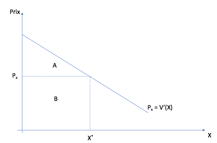
The area A+B is given by $V(X^*) - V(0)$ while area B is expenditures $p_{X}X^*$. Therefore consumer surplus is A+B - B = A.¶

Exercise B: If $V(X) = 10 X - \frac{1}{2}X^2$, find the expression of consumer surplus.

Welfare and Taxation¶

Taxation impacts the price paid by the consumer. Therefore, it has effects on welfare (since higher prices lower welfare). Compensated income will help quantify the welfare loss from higher prices (or taxes).

Consider eliminating a tax, the price decreases from $p_X = p+t$ to $p_X = p$ . We have $X^*(p) > X^*(p+t)$ (we are not in a Giffen good situation). Income from the tax is $T= t X^*(p+t)$. When the government collects a tax, we assume that the revenues are distributed lump-sum (an amount for each consumer, not dependent on actions). From a welfare point of view, revenue collected from the government is not lost (implicitly it funds services, etc). Here we recognize its cash value.

In terms of compensating variation, we have

\[\Delta I^{CV} = U[X^*(p), I - pX^*(p)] - U[X^*(p+t), I - (p+t) X^*(p+t)] > 0\]

We obtain that $\Delta I^{CV} > T$: The consumer is willing to pay an amount which is superior to the revenue generated by the tax. Hence, eliminating the tax is beneficial.

The welfare gain associated with eliminating the tax is therefore $\Delta W = \Delta I^{CV} - T$. Why is $T$ subtracted? Removing the tax, the government cannot redistribute anymore the proceeds lump-sum. Hence, we have to subtract it from the change in consumer surplus. If we introduce a tax, we have $\Delta W = \Delta I^{CV} + T$ since we need to redistribute the tax proceeds lump-sum, which is gained for consumers.

Exercise C: If $V(X) = 10 X - \frac{1}{2}X^2$, find the welfare loss associated with a new tax $t$ on good $X$. Show this loss graphically.

Welfare and Air Quality¶

Generally, consumers have a positive preference for air quality.

There is no market for air quality. With the Clean Air Act (1977), the American government has put in place a number of regulations which reduce pollution and improve air quality.

Consider a policy change from $\mathcal P_0$: no control and costs, to $\mathcal P$: pollution controls and costs. The compensating variation should be positive for consumers if they value air quality.

Empirically, how can recover such a preference?

We can aim to find a situation where consumers had to face a trade-off between pollution and income (wealth). For example, the decision to purchase a home may depend on the price of the home but also air quality of the neighborhood. Price and air quality vary inside a city. In a market, prices should be higher if air quality is higher if consumers value air quality.

Using data from real estate transactions, we can determine the value given to air quality. Define $X$ as air quality, (e.g. air particule concentration) We might want to assume preferences are given by:

\[U(X, Y) = V(X) + Y = \alpha X + \beta X^2 +Y\]

With this utility function $V'(X)$ represents a willingness to pay for air quality. Running a linear regression real estate transaction amounts on $X$ controlling for other factors, we obtain an estimate of $V'(X)$.

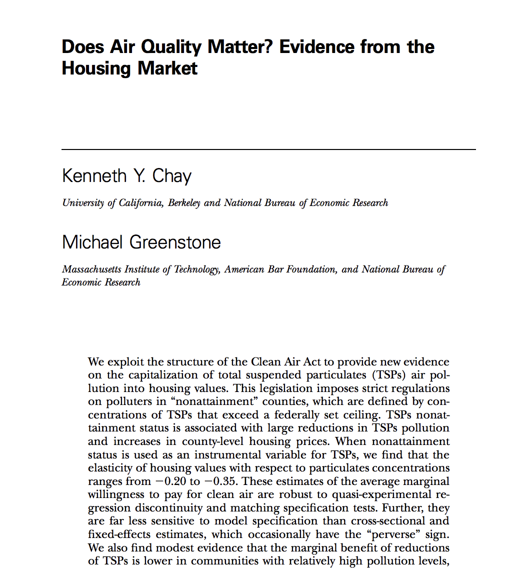
Chay et Greenstone (2005) obtain a price-particle elasticity between -0.2 and -0.35.

Now, how do we evaluate a policy with this information? The government implements $X_{GOV}$. The total cost of these measures is $c X_{GOV}$ where $c>1$ is the marginal cost, including the welfare loss from raising this amount of revenue to fund these measures.

The policy change is from $(0,0)$ to $(X_{GOV}, - c X_{GOV})$. Consumer surplus is the compensating variation:

\[\Delta I^{CV} = V(X_{GOV}) - V(0) - c X_{GOV} .\]

This serves as a basis for performing cost-benefit analysis. Once this analysis is done, a follow-up question to ask is: what is the optimal amount of air quality?

Optimal air quality is the level which maximizes

\[U(X) = V(X) + I - c X\]

The FOC is

\[V'(X^*) = c\]

We can therefore find out this optimal level once we know these qualities.

Exercise D: Noise pollution. The price elasticity of house prices to noise pollution is -0.2. The government considers reducing pollution by 10% near a highway. Engineers estimate the necessary technology will cost 1000$ per house protected (a sound wall). The policy is financed by a tax, which leads to a welfare loss of 43 cents for each dollar that needs to be raised. Would building the sound wall be beneficial in terms of welfare?

This approach is used a lot. It does not require per se knowledge of preference. However, it raises a number of distributive issues if preferences differ across consumers. When the benefits are larger than the cost, but some loose from the policy, we say that the policy is potentially beneficial, implying that compensation may need to take place.

Self-Reported Happiness¶

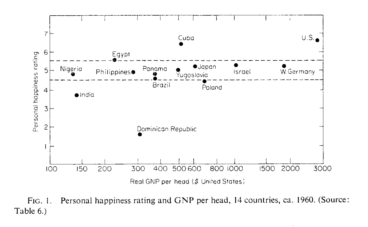
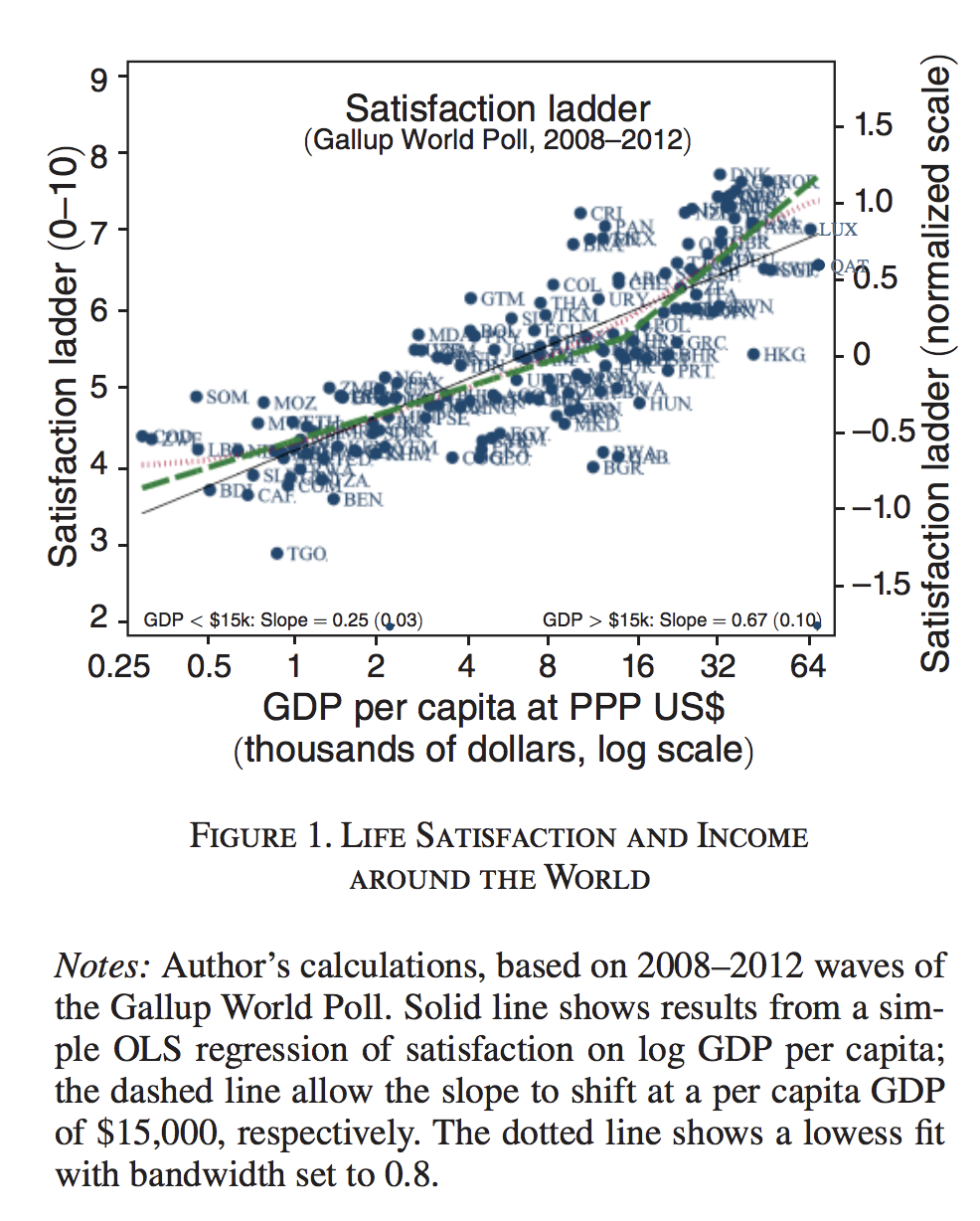
Why not simply ask consumers of they are happy, or happier after a policy change? On a scale of 1 to 10, are you happy? This avoids making assumptions about preferences, utility. It is an approach that has gained credibility with the 2019 budget in New Zealand. Richard Easterlin is generally credited with making these measures popular. The Easterlin paradox has attracted a lot of attention.

This would suggest that we are not happier with more income: money does not buy happiness. But later, with more data, the expected relationship was shown to hold, in particular for low levels of income.

Stevenson and Wolfers (2013), AER: Papers and Proceedings¶

Since happiness is more than income, these measures can be useful. One could use them directly in policy evaluation:

Advantages: direct method, model free.
Disadvantages: We can measure welfare in different ways and people have different ways of answering. Various psychological and framing effects possible.

Few studies use them. But there is a lot of interest, for good reasons.

For those who want to go deeper, here is an interview with Angus Deaton on happiness: