Introduction
Theory and Data
The website missingprofits.world computes what each country loses to tax heavens. But how do we reform the tax system so that profits are taxed? What effects would a wealth tax have on inequality? How much revenue could it generate?
We need micro theory to understand incentive effects created by taxes. We also need data. Economists like Emmanuel Saez and Gabriel Zucman study these questions with data and theory.

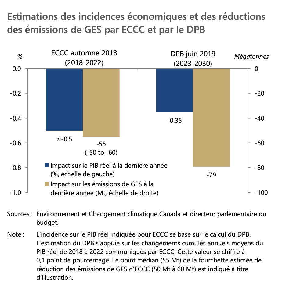
A carbon tax could be effective to reduce emissions. But what are the effects of such taxes on the economy? In 2019, the Parlementary Budget Office of Canada wrote a report which uses an economic model to compute these effects. The model combines data and theory.
How should we set up the market for advertising on the internet? What is the price of information? How should we price rankings in search engines? Hal Varian is the chief economist at Google. He is also the author of a well-known micro theory book. In his everyday work, he combines theory and data to help companies in the new economy. See this interview with him.
Data is everywhere. Theory helps make sense of it:
To understand behavior
To quantify effects of policies and assess them
Pricing and optimization in firms
This article from Judea Pearl, a pioneer in AI, warns of the dangers of using data without theory (in his words, cause to effect mechanisms).
Mathematical Toolbox
Math is essential to understand behavior, measure effects of changes in the environment (e.g. prices and taxes). Here is a explainer on a number of key tools we will be using.
Marginal Analysis and Approximations
How do we describe a function \(f(x)\)?
Functions can be complicated, can be approximated by linear functions for small perturbations…
Locally, we can do an approximation of a smooth function for \(x\) close to \(x_0\):
\[f(x) \simeq f(x_0) + \alpha (x-x_0)\]
To best the best \(\alpha\), we have that for \(x\) close to \(x_0\)
Where \(f'(\cdot)\) is the first derivative of the function \(f(\cdot)\). So,
If we want to predict the change in a function for a small change in its argument, the derivative is the best way to do it…
Derivatives
With constants
\(f(x) = b + ax\): \(f'(x) = a\)
\(f(x) = \log x\): \(f'(x) = \frac{1}{x}\)
\(f(x) = e^{ax}\): \(f'(x) = ae^{ax}\)
\(f(x) = x^a\): \(f'(x) = a x^{a-1}\)
With functions
Product rule: \(f(x) = a(x)b(x)\), \(f'(x) = a'(x)b(x) + a(x)b'(x)\)
Quotient rule: \(f(x) = \frac{a(x)}{b(x)}\), \(f'(x) = \frac{a'(x)b(x) - a(x)b'(x)}{b(x)^2}\)
Chain rule: \(f(x) = a(b(x))\), \(f'(x) = a'(b(x))b'(x)\)
Addition (substraction) rule: \(f(x) = a(x) + b(x)\), \(f'(x) = a'(x) + b'(x)\).
Exercise A: Find the first derivative of : \(f(x)=\sqrt{x},\frac{x}{1+x},\frac{1}{2}x^2 + 2x-10,(1+\frac{x}{2})^2\).
Exercise B: Compute a first-order approximation of \(f(x)=\sqrt{x}\) around \(x_0\).
Higher Order Approximations
We can compute higher-order derivatives. The second derivative is the first derivative of the first derivative, etc. If these higher-order derivatives are not zero, we can improve the approximation of the function for small perturbations.
We denote \(f'(x), f''(x)\) or \(\frac{d f}{d x},\frac{d}{d x}(\frac{d f}{d x}) = \frac{d^2 f}{d x^2}\) the second derivative of a function. In this course, you will not need to go above second derivatives.
Concavity and Convexity of Functions
A function is concave if for all (pair of) points, \((x_1,x_2)\) and all \(0<\lambda<1\):
and convex if false. We say strictly concave (or convex) if these inequalities are strict. The second derivative is useful for concavity and convexity. A function is strictly concave is the second derivative is negative for all points, and strictly convex if positive for all points.
Approximation and Optimum
Consider the first order approximation
We have that if:
\(f'(x_0)>0\), a small change \(\Delta x>0\) increases \(f\)
\(f'(x_0) <0\) a small change \(\Delta x <0\) increases \(f\)
\(f'(x_0) =0\), then \(x_0\) is the solution to \(\max_x f(x)\).
This last first order condition (FOC) is necessary for an optimum. We need the first derivative to be zero at the optimum.
The FOC is not sufficient. We also need a second condition, i.e. that the second derivative is negative. Here we skip the details, but this avoids inflection points, where the FOC is satisfied but where we do not have a maximum or a minimum.
Exercise C: Find the maximum for the function \(f(x) = x(10-x)\).
Partial Derivatives
Consider the function \(f(x,y)\). The partial derivative changes one variable, keeping the others fixed: \(f'_x(x,y) = \frac{\partial f(x,y)}{\partial x}\).
Total Differentiation
Sometime, it makes sense to look at combinations of \((x,y)\) that keep the function fixed to some value \(f(x,y) = \overline{f}\). We can invert the function, \(y=g(x,\overline{f})\). But, we can also use total differentiation which exploits linear approximations.
We can perturb a function starting at a point and this equation holds
The operator d denotes a change. If we set \(df(x,y)=0\), we can rearrange to obtain.
We add \(df=0\) to indicate that it is a derivative, keeping the value of the function fixed.
Exercise D: Find \(\frac{dy}{dx}\Bigr|_{df=0}\) using total differentiation \(f(x,y)=\log(xy)\).
Homogeneity of a Function
A partial derivative provides information of how a function changes when we change one variable, keeping others fixed. But sometimes we want to understand how a function changes when all its variables change in the same proportion. Just like we want to know whether if we double a recipe for a cake, we get two cakes, or something else. This is called the degree of homogeneity of a function. There are two ways to proceed:
Direct approach: A function is homogeneous of degree \(r\) if for all \(\lambda>0\),
Euler Theorem: If a function is homogeneous of degree \(r\), then:
Exercise E: Find the degree of homogeneity of the function \(f(x,y)=x^\alpha y^\beta\) using both methods.
Maximum and Approximation
We need as many first-order conditions as there are variables we maximize over. The necessary conditions are
\(f'_x(x,y)=0, f'_y(x,y)=0\)
for a function \(f(x,y)\). The second order conditions are a bit more complicated and we do not cover it here.
Constrained Maximization
A constrained problem takes the form:
Direct approach
If we can invert \(g(x,y)=m\) to get a function \(y=q(x,m)\), then the solution of the constrained problem for \(x\) is the same the solution to the unconstrained problem:
For the FOC is \(f'_x(x,q(x,m)) + f'_y(x,q(x,m))q'(x,m) = 0\). We can solve for \(x^*\) and use \(y=q(x)\) to find \(y^*\).
Exercise F: Maximize the function \(f(x,y) = \log x + \log y\) subject to the constraint \(x+y \le m\).
With more than 2 variables and many constraints, this approach is not practical…
The Lagrangian
The method proposed by Lagrange is to solve for the pair \((x,y)\) using the set of three conditions:
Where \(\lambda\) is a Lagrange multiplier.
If we think backwards, these three equations are the first order conditions to the Lagragian:
The Lagrangian \(L(x,y,\lambda)\) is a modified objective function which penalizes the constraint added to the unconstrained maximization of the objection function. If \(\lambda = 0\), the first two FOC above are the unconstrained FOC, \(f'_x(x,y)=0\) and \(f'_y(x,y)=0\) which yield the unconstrained optimum. If one of the constraints is binding (if \(\lambda \neq 0\)) will we get a different solution.
Exercise G: Maximize the function \(f(x,y) = \log x + \log y\) under the constraint \(x+y \le m\) using a Lagrangian.
Note on logs
In these notes, we use \(\log\) to denote the logarithm with base \(e=2.718281828459\) and not base 10. So, it is the natural log (\(\ln = \log_e\)). Python also uses this base in the numpy library.