Price and Income Effects
Does a tax on gasoline decrease gas consumption and promotes public transportation?
To answer a question like this, we need to study empirically how the demand for gasoline and public transportation respond to a tax. A tax results in a price change for the consumer. Hence, a prerequisite is that we study how demand responds to price. Second, we may want to compensate individuals for the burden of the tax. For this, we need to know how demand changes as a function of income. Related to this is the question of whether or not such taxes are regressive or not.

The gilets jaunes in France in part demonstrated because of new gasoline taxes which they argued reduced their purchasing power.
Price and income elasticity can be estimated without theory. But theory is necessary to answer the more normative questions and to talk about compensation.
Demand and Preferences
Let us formalize the problem above:
Gasoline (\(X\)) et Public transporation (\(Y\))
Preferences may be represented by \(U(X,Y)\). We will assume all consumers have the same preferences.
Budget constraint: \(p_X X + p_Y Y \leq I\)
Demand functions are \((X^*, Y^*)\) such that
At the optimum, the budget is spent and the consumer is indifferent between reducing or increasing \(X\) and \(Y\).
We have two equations in two unknowns: the solution for \(X^*\) and \(Y^*\) as a function of \((p_X,p_Y,I)\) give the marshallian demands.
Example
For preferences represented by \(U(X,Y) = \log X + 2\log Y\),
One can use \(p_X X + p_Y Y = I\) to obtain
The question is how to characterize how \(X^*\) et \(Y^*\) change as a function of \(I\) and prices?
Income Effects
We start with variation of income.
Engel Curves
The consumer demands \(X(p_X,p_Y,I)\) and \(Y(p_X,p_Y,I)\).
The Engel curve for \(X\): How \(X^*\) changes when \(I\) change?
There is a version which also looks at the relationship between the budget share of \(X\), \(s_X = \frac{p_X X}{I}\) as a function of income.
Normal Good
A good is normal if and only if the quantity demanded increases with income (at constant prices).
Inferior Good
A good is inferior if its demand decreases when income increases (at constant prices).
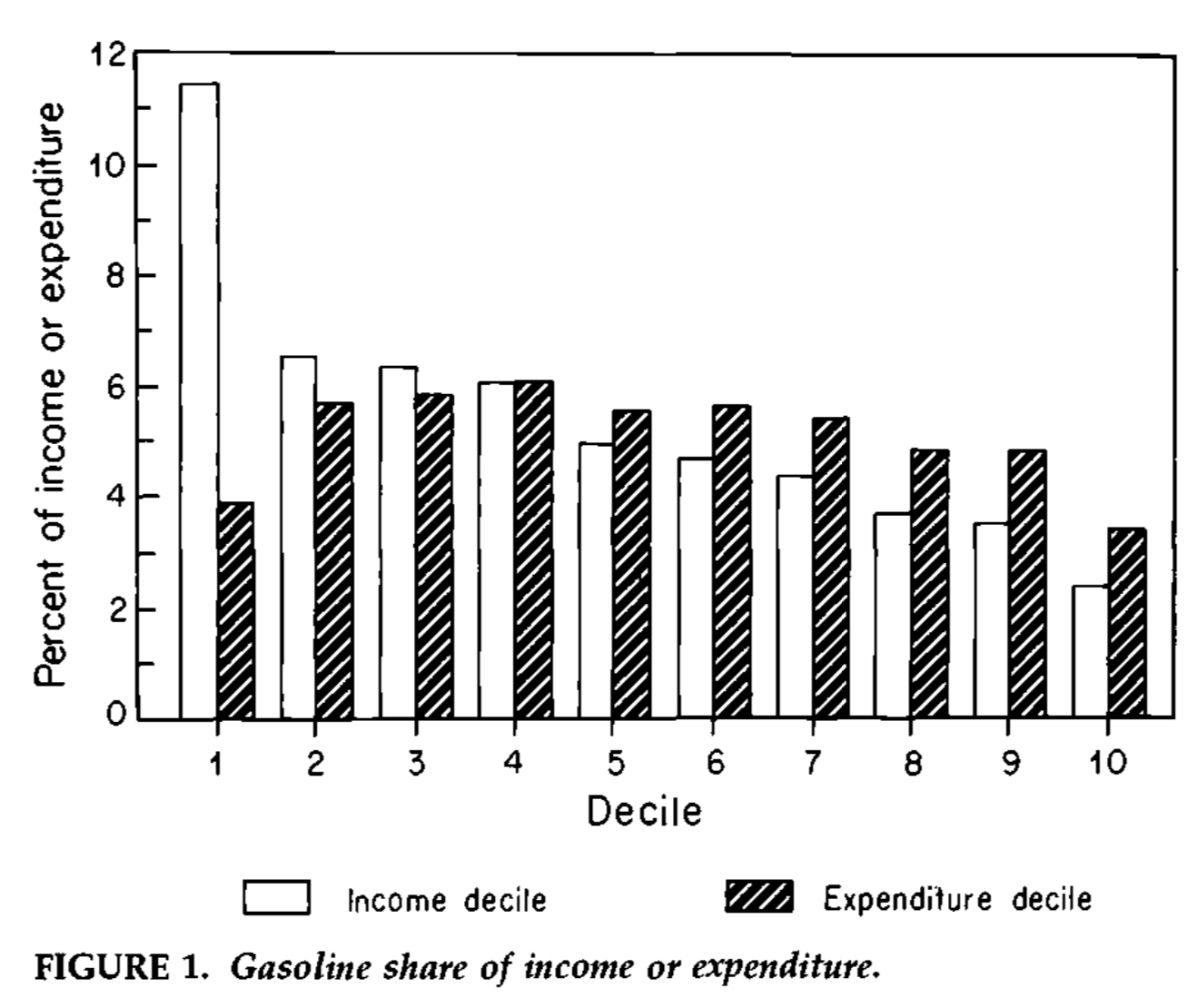
Is gasoline an inferior or normal good? One study by James Porterba ((Poterba, 1991)) suggests that it is inferior if we look at income but not if we look at spending. The reason has to do with variation in spending from savings.
To quantify income effects, we can use an income elasticity defined as
In practice, it is hard to observe the income elasticity because variation in income is rarely exogenous. What sort of events could you exploit?
Price Effects
How do the demands \(X^*\) et \(Y^*\) change if \(p_Y\) and \(I\) stay constant but \(p_X\) changes?
To quantify this margin, we may use a price elasticity of the form:
This elasticity is invariant to monetary units. A challenge is to find an experiment where the price is varied exogenously while other factors are kept constant. Taxation is one of the key margins exploited. Other examples include supply shocks.
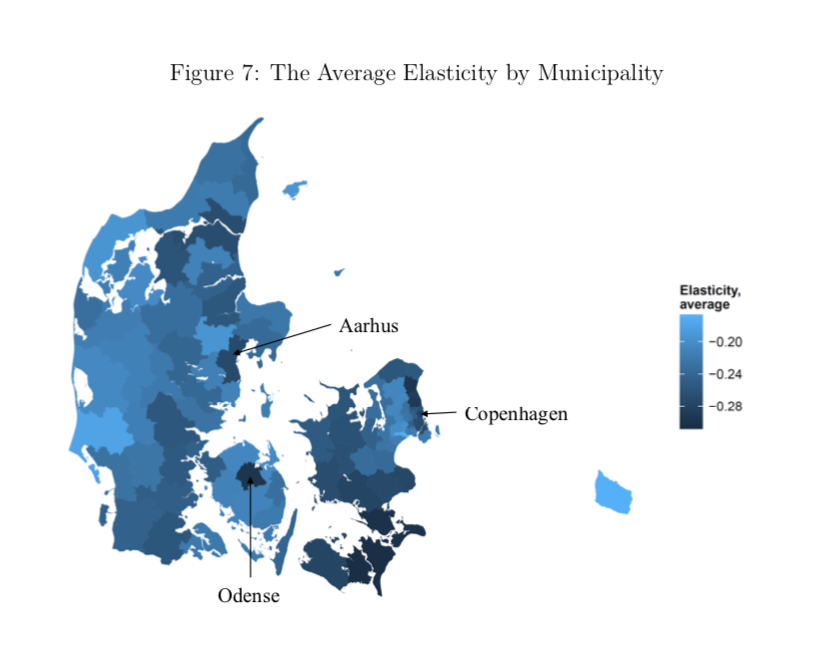
In Denmark, one study shows that the price elasticity varies a lot across the country and in particular reacts to the distance people need to travel to work and transportation alternatives they face.
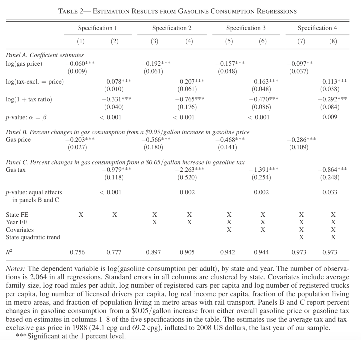
In the U.S., another analysis shows that a distinction should be made between a price change and a tax change. The effect of a tax appears to be more visible and people react more to it.
What are the implications for tax revenue? Hint: Think of the effect of the elasticity on tax revenue.
An increase in the price (or tax) has a direct effect of lowering utility. One may want to compensate households for this. To compute the compensation, we have to think of the forces of what leads to a behavioral change.
There are two forces:
Public transportation is more affordable than the car (gasoline): consumers will want to substitute towards public transportation. This is a substitution effect which comes from the relative price signal.
\[\frac{U'_X(X,Y)}{U'_Y(X,Y)} = \frac{p_X}{p_Y}\]At current consumption, one needs more income to buy this basket at the new prices. Hence, the consumer needs to reduce his consumption: income effect.
Compensation will be a function of income and substitution effects. Hence, our objective: is to identify these effects and see how they lead to the total price effect.
Compensated Demand
Compensated demand allows to separate substitution and income effects.
Context
Reference price \((p_X,p_Y)\), reference income \(I\)
New prices \((\hat p_X,p_Y)\), income does not change.
Reference Demand, \(X(p_X,p_Y,I)\), indirect utility level at reference price and income \(V(p_X,p_Y,I)\)
New Demand, \(X(\hat p_X, p_Y, I)\), new indirect utility level \(V(\hat p_X,p_Y,I)\).
Compensated Income: income \(I^{cmp}\) such that we maintain utility at reference levels despite facing new prices.
\[V(p_X,p_Y, I) = V(\hat p_X, p_Y, I^{cmp})\]
Compensated demand (or hicksian) is given by the marshallian demand where we replace income by compensated income \(X^{cmp}= X(\hat p_X, p_Y, I^{cmp})\). There exist a dual theory of consumer choice which alternatively derives the compensated demand from minimizing expenditures subject to maintaining utility above a certain level. We do not do this here.
Compensated income for a price increase is always higher than reference income. The difference is the compensation required. If the price increase results from a tax, this new compensation is required not to make consumers worse off. Yet, even if the compensation occurs, it still has the potential of changing behavior: a price change results in a potential substitution effect which does not go away if compensation occurs.
Law of Compensated Demand If \(\hat p_X > p_X\), then \(X^{cmp}(p_X,p_Y,I)<X(p_X,p_Y,I)\). Compensated demand for \(X\) is decreasing in the price \(p_X\).
Exercise A: Compute compensated income and demand for \(X\) if \(U(X,Y) = XY\) and \(p_XX+p_YY \le I\) for a price change \(\hat p_X > p_X\).
We can now define substitution and income effects.
Substitution Effect
Change in demand caused by a relative price change, keeping utility constant.
Substitution Effect \(=\) Compensated Demand - Reference Demand
\[\Delta X^{{cmp}} = X(\hat p_X,p_Y,I^{cmp}) - X(p_X,p_Y,I)\]
Income Effect
Change in demand caused by a change in purchasing power, keeping prices constant.
Income Effect \(=\) New demand - compensated demand
We can approximate the compensated income for a small change in price:
\(\hat p_X = p_X + \Delta p_X\).
To keep notation light, denote
\(X^* = X(p_X,p_X,I)\), \(Y^* = Y(p_X,p_Y,I)\)
Then define \(I^{cmp}= I + \Delta I^{cmp}\), \(X^{cmp}= X^* + \Delta X^{cmp}\) and \(Y^{cmp}= Y^* + \Delta Y^{cmp}\).
Therefore,
Why does \(p_X\Delta X^{{cmp}} + p_Y \Delta Y^{{cmp}} = 0\)?
\((X^*,Y^*)\) and \((X^{cmp},Y^{cmp})\) are on the same indifference curve and close to each other for a small price change, which implies,
\[\frac{\Delta Y^{cmp}}{\Delta X^{cmp}} = MRS_{X}\]
\((X^*,Y^*)\) is optimal at prices \(p_X, p_Y\), which implies \(MRS_{X} = -\frac{p_X}{p_Y}\).
Therefore, \(p_X \Delta X^{cmp}+ p_Y \Delta Y^{cmp}= 0\).
Exercise B: See if this is a good approximation for \(U(X,Y) = XY\) with reference price and income \((p_X,p_Y,I) = (1,1,100)\) and \(\Delta p_X = 1\). Redo the exercise for \(\Delta p_X = 0.1\).
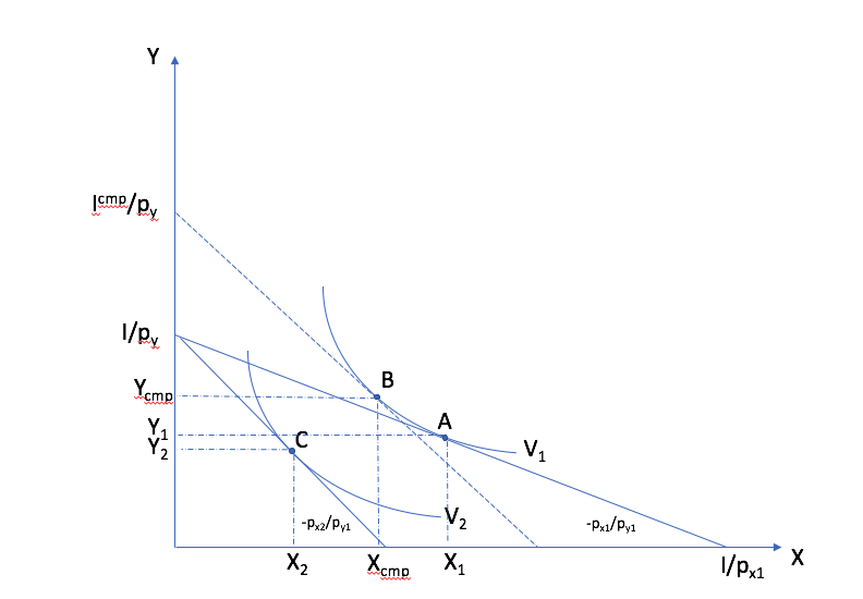
In the \((X,Y)\) space, consider a price increase for good \(X\). The index 1 refers to the reference situation and index 2 to the situation with the new prices. The consumer is initially at point A (reference). With the price change, the budget constraint has a steeper slope. After the price change, the consumer is at price C. To decompose this price change, we compensate the consumer at the new prices. He chooses point B, with the same utility as in the reference situation. The passage from A to B is the substitution effect. The passage from B to C is the income effect. The sum of the two yield the total effect of the price change.
Slutsky Equation
The Slutsky equation allows to look the total price effect, the substitution effect and the income effect. The first and the last is observable given sufficient exogenous variation. The second one is necessary to compute the compensation required.
To keep notation simple, consider
We get
Exercice C: Find the substitution and income effects in exercise B (\(\Delta p_X = 1\)).
Since
then,
In terms of elasticities,
The Slutsky equation becomes:
Exercice D: For Cobb-Douglas preferences \(U(X,Y) = X^\alpha Y^{1-\alpha}\), compute compensated price elasticity using the Slutsky equation.
Cross-price Effects
Let us first talk about the nature of goods, complements or substitutes. Turns out compensated demands are necessary to define those precisely. Goods \(X\) and \(Y\) are:
Substitutes: if the cross-price effect is positive: \(\frac{\partial X^{cmp}}{\partial p_Y} >0\)
Complements: If the cross-price effect is negative: \(\frac{\partial X^{cmp}}{\partial p_Y} <0\)
What is your prior about the cross-price elasticity of public transportation? How would it factor into your analysis of a policy that taxes gasoline to reduce carbon emissions?
Properties of Demand Functions
Homogeneity of degree zero (no monetary illusion)
\[X(\lambda p_X,\lambda p_Y,\lambda I) = X(p_X,p_Y,I)\]Symmetry:
\[\frac{\partial X^{cmp}}{\partial p_Y} =\frac{\partial Y^{cmp}}{\partial p_X}\]Additivity:
\[p_X \frac{\partial X(p_X,p_Y,I)}{\partial I} + p_Y \frac{\partial Y(p_X,p_Y,I)}{\partial I} = 1\]Negativity (Law of compensated demand):
\[\frac{\partial X^{cmp}}{\partial p_X}<0,\frac{\partial Y^{cmp}}{\partial p_Y}<0\]
Price indices of cost-of-living
To measure how the cost-of-living changes, we use consumer price indices (CPI). One such index is the Laspeyres index:
Note that \(X\) and \(Y\), bought in the reference situation, are also used after the price change. This CPI keeps quantities fixed, at least in the short term. The policy question is that many government benefits are indexed to the CPI and it is not clear whether the CPI really reflects changes in purchasing power. The objective of this indexation is to maintain power purchasing power of these benefits constant but it does not account for the fact that consumers substitute away from goods whose price increases more, in relative terms. Another issue is that monetary policy is also based on inflation which is measured using the CPI.
For an increase in the price of \(X\), the effect on purchasing power can be measured with:
\[\pi_I = \frac{I^{cmp}}{I}\]
This will depend on preferences. It is possible that this Hicksian price index yields a different answer than the Laysperes price index. In particular, if the income share of a good decrease when its price increase, the Hicksian index often yields a lower increase in the cost-of-living than what the Laysperres index would suggest. We call this bias the substitution bias in price indices.
Before the pandemia hit and a lockdown was imposed, gasoline consumption went down. The price of gas also decreased (for may reason). Does a Laysperes index give a good indication of the change in purchasing power during this period? This article does the computation for the U.S. and shows that inflation is underestimated.
Giffen Goods
There exist a type of good for which demand increases with the price! Look back at the Slutsky equation:
The first term is always negative. This comes from the Law of compensated demand… To get a positive elasticity, we therefore need the second term to be negative (so that it becomes positive when subtracted).
A necessary condition is therefore that the good is inferior \(\eta_{X,I}<0\). But to overcome the negative substitution effect, this is not sufficient. We need this negative income effect to be large and (or) the budget share to be large.
So, it is possible that \(\eta_{X,p}>0\). But do we see this case in reality? (read the story behind Giffen goods on wikipedia). The best example we know comes from China. A subsidy program for rice was introduced, bringing down the price (Jensen et Miller (2008)). This leads to a reduction in rice consumption.
Firm pricing and demand analysis
Why would a firm study properties of the demand it faces? Because it can potentially increase sales if it has market power, an ability to affect or manipulate the price on the market. Firms can also price discriminate: segment the market or offer bundles at different prices. They can exploit complementarities between goods to offer bundles. All of this requires good knowledge of demand.
Econometric analysis can be used along with some theory, to extract information from firm and market data. In the retail industry, firms purchase for example scanner data to learn about consumers and their sensitivity to prices.
Python example
See this notebook which uses the CES utility function to study price and income effects.
![]()